Programming and Backtesting Demonstrations for a Buy-Sell Model for Eight Tickers
A prior blog post introduced building and backtesting a buy-sell model for a pair of tickers (SPY and SPXL). The prior post demonstrated how to manually implement and backtest the model in a Google Sheets worksheet. The current blog post illustrates how to build key elements of the model programmatically for eight tickers (SPY, SPXL, QQQ, TQQQ, MSFT, NVDA, GOOGL, and PTIR). Programming the model makes it easier and faster to evaluate more tickers and more time periods than with manual data processing. The programming for this post is implemented with T-SQL, the SQL Server scripting language. After implementing the model programmatically, this post demonstrates how to backtest model outcomes for different tickers in a Google Sheets worksheet. The backtest analyses in this post are more detailed than in the prior blog post because the programmed version of the model makes it easier to process more data and provide it in a format that facilitates more thorough backtesting.
The model evaluated in this post relies on the relationship between close prices and exponential moving averages (EMAs). A single set of close prices for a ticker can have multiple EMA series -- each with a different period length parameter. EMAs with a shorter period length parameter reflect short-term close price changes better than EMAs with a longer period length parameter. Conversely, EMAs with a longer period length parameter reflect long-term close price trends better than EMAs with a shorter period length parameter.
The model in this post uses two EMAs – one with a period length of 10 days and another with a period length of 200 days. The prior blog post describes and demonstrates how to download close prices from the Google Finance site into a Google Sheets worksheet for a ticker as well as how to compute EMAs series with period lengths of ten-periods (EMA_10) and two-hundred-periods (EMA_200). Identical pre-processing steps were performed to prepare data for modeling in this post. See the prior blog post for detailed steps on how to perform the pre-processing steps.
The Model and the T-SQL Code for Implementing It
EMAs are a smoothing technique for time series data, such as the close prices for a ticker over a range of trading dates. When the underlying close price increases from one period to the next period, both the EMA_10 and EMA_200 series values rise. If the underlying close price decreases from one period to the next period, both the EMA_10 and EMA_200 series values decline. A third possible outcome is for there to be no change for one period to the next.
The model implemented and analyzed in this post depends on these relationships to determine when it is a profitable time to own the underlying security for a ticker. When the close prices in a set of consecutive periods are greater than their corresponding EMA_10 and EMA_200 values, then it is a profitable time to own a security because both close prices and their corresponding EMA values are in an uptrend.
Close prices can change their direction in a run of consecutive periods with the same relationships between close prices and EMAs. However, so long as the close price for a period is above its EMA_10 and EMA_200 values, then the close price is in an uptrend relative to its prior close price. When the close value is below either its EMA_10 or EMA_200 values, then the close, EMA_10, and EMA_200 values are not in an uptrend.
Here is a summary of the following T-SQL code to process the daily underlying ticker close prices and their corresponding EMA values for a backtesting analysis. It is not necessary for you to understand the code in order to grasp the main takeaways from this post, but learning how the code works will help you to build your own automated model building skills for other tickers beyond those examined in this post.
- The code starts by creating a fresh copy of the FinancialData table in the SecurityTradingAnalytics database (you can use any other database to which you have access through the programming language that you use to implement the model). The initial version of the FinancialData table has seven columns (Ticker, Date, Close, EMA_10, EMA_30, EMA_50, and EMA_200). The EMA_30 and EMA_50 columns are included to encourage you to implement the model with other EMA series besides the two analyzed in this post.
- The next major step is to populate the FinancialData table with values from the “For Copy to SS ver 3.csv” file. This file contains historical data for backtesting the model. By substituting a custom version of this file for the one analyzed in this post, you can build and backtest the model for different tickers and historical datasets besides those analyzed in this post.
- An alter table statement updates the FinancialData table with a computed column named CloseAboveEMA. The code for this column returns row values of TRUE or FALSE. The return value is TRUE when the close price for a trading day is greater than the EMA_10 and EMA_200 values for a trading day. Otherwise, the returned CloseAboveEMA value is FALSE. When the returned CloseAboveEMA value is TRUE, the close price ends the trading day in an uptrend, indicating the day is a profitable one to own the underlying security for a ticker.
- Next, two common table expressions (CTEs) with trailing query statements create and populate the #temp_FirstDate_LastDate and #temp_FirstClose_LastClose temp tables. For each Ticker, both temp tables contain RunGroup identifier values for denoting the consecutive set of trading days to which each trading day belongs.
o Consecutive rows in the FinancialData table can be either of two types: those with a CloseAboveEMA value of TRUE or those with a CloseAboveEMA value of FALSE.
o The expression for the RunGroup column values in the CTEs define unique identifier values for alternating sets of rows with TRUE CloseAboveEMA values versus FALSE CloseAboveEMA values.
o The rows in each of the two temp tables contain one row per Ticker and Rungroup.
- The next-to-final block of code in the following script joins the #temp_FirstDate_LastDate and #temp_FirstClose_LastClose temp tables and adds two additional columns to the joined results set, which is stored in the #temp_summary table.
o The first added column has the name Close Change. It is computed as LastClose value less FirstClose value for each row in the #temp_summary table.
o The second added column has the name LastClose/FirstClose. Each row for this column has the ratio of the LastClose value divided by the FirstClose value from the joined results set.
o The rows of the #temp_summary table are ordered by Ticker and RunGroup column values.
- The final block of code returns eight results sets – one for each of the Ticker values in this post. At the conclusion of the model implementation, the backtest analysis copies the results set for each ticker to a separate tab in a Google Sheets worksheet. If you wish to adapt the following script to collect results for a different collection of tickers, you will need to replace the ticker values in this section with the new tickers you are analyzing. The process for implementing the backtest is described and illustrated in the next section of this post.
-- designate a database into which to insert the table
use SecurityTradingAnalytics
go
-- conditionally drop FinancialData table
-- if it already exists
IF OBJECT_ID('dbo.FinancialData', 'U') IS NOT NULL
DROP TABLE dbo.FinancialData;
CREATE TABLE FinancialData (
Ticker NVARCHAR(50) NOT NULL,
Date DATE NOT NULL,
[Close] DECIMAL(18, 2),
EMA_10 DECIMAL(18, 2),
EMA_30 DECIMAL(18, 2),
EMA_50 DECIMAL(18, 2),
EMA_200 DECIMAL(18, 2)
)
ALTER TABLE dbo.FinancialData
ADD CONSTRAINT PK_FinancialData_Ticker_Date PRIMARY KEY (Ticker, Date);
-- returned t-sql for: show me bulk insert statement for populating
-- FinancialData table from C:\Users\Public\Downloads\For Copy to SS ver 3.csv path
-- It was convenient to rename file name for downloaded csv file from Google Sheets
BULK INSERT FinancialData
--FROM 'C:\Users\Public\Public Downloads\For Copy to SS ver 3.csv'
FROM 'C:\Users\Public\Downloads\from_google_sheets.csv'
WITH (
FORMAT = 'CSV', -- Specifies that the file is in CSV format
FIRSTROW = 2 -- Skips the header row
);
-- optionally echo freshly populated table
-- select * from FinancialData
-- select count(*) from FinancialData
-- select ticker, count(*) from FinancialData group by ticker
-- t-sql to return a computed column with TRUE or FALSE
-- values based on the relationship of close prices to ema values,
-- such as ema_10 and ema_200
ALTER TABLE FinancialData
ADD CloseAboveEMA AS
CASE
WHEN [Close] > EMA_10 AND [Close] > EMA_200 THEN 'TRUE'
ELSE 'FALSE'
END;
-- conditionally drop a temp table named #temp_FirstDate_LastDate and
-- a temp table named #temp_FirstClose_LastClose
IF OBJECT_ID('tempdb..#temp_FirstDate_LastDate') IS NOT NULL
BEGIN
DROP TABLE #temp_FirstDate_LastDate
END;
if object_id('tempdb..#temp_FirstClose_LastClose') is not null
begin
drop table #temp_FirstClose_LastClose
end;
--go
-- t-sql code to return FirstDate and LastDate
-- by Ticker and RunGroup in #temp_FirstDate_LastDate
WITH NumberedRuns AS (
SELECT
Ticker,
[Date],
CloseAboveEMA,
ROW_NUMBER() OVER (PARTITION BY Ticker ORDER BY [Date]) -
ROW_NUMBER() OVER (PARTITION BY Ticker, CloseAboveEMA ORDER BY [Date]) AS RunGroup
FROM FinancialData
)
SELECT
Ticker,
RunGroup,
MIN([Date]) AS FirstDate,
MAX([Date]) AS LastDate
into #temp_FirstDate_LastDate
FROM NumberedRuns
WHERE CloseAboveEMA = 'True'
GROUP BY Ticker, RunGroup
ORDER BY Ticker, RunGroup;
-- optionally echo values in #temp_FirstDate_LastDate
-- select * from #temp_FirstDate_LastDate order by Ticker, RunGroup
-- t-sql code to return FirstClose and LastClose by Ticker and RunGroup
-- in #temp_FirstClose_LastClose
WITH NumberedRuns AS (
SELECT
Ticker,
[Date],
[Close],
CloseAboveEMA,
ROW_NUMBER() OVER (PARTITION BY Ticker ORDER BY [Date]) -
ROW_NUMBER() OVER (PARTITION BY Ticker, CloseAboveEMA ORDER BY [Date]) AS RunGroup
FROM dbo.FinancialData
)
SELECT DISTINCT
Ticker,
RunGroup,
FIRST_VALUE([Close]) OVER (PARTITION BY Ticker, RunGroup ORDER BY [Date]) AS FirstClose,
LAST_VALUE([Close]) OVER (
PARTITION BY Ticker, RunGroup
ORDER BY [Date]
ROWS BETWEEN UNBOUNDED PRECEDING AND UNBOUNDED FOLLOWING
) AS LastClose
into #temp_FirstClose_LastClose
FROM NumberedRuns
WHERE CloseAboveEMA = 'True'
ORDER BY Ticker, RunGroup;
-- optionally echo values in FinancialData,
-- #temp_FirstDate_LastDate, and #temp_FirstClose_LastClose
-- select * from FinancialData
-- select * from #temp_FirstDate_LastDate order by Ticker, RunGroup
-- select * from #temp_FirstClose_LastClose order by Ticker, RunGroup
-----------------------------------------------------------------------------------------------
-- code to join #temp_FirstDate_LastDate and #temp_FirstClose_LastClose
-- plus two computed columns named [Close Change] and [LastClose/FirstClose]
if object_id('tempdb..#temp_summary') is not null
begin
drop table #temp_summary
end;
--go
select
#temp_FirstDate_LastDate.Ticker
,#temp_FirstDate_LastDate.RunGroup
,#temp_FirstDate_LastDate.FirstDate
,#temp_FirstDate_LastDate.LastDate
,#temp_FirstClose_LastClose.FirstClose
,#temp_FirstClose_LastClose.LastClose
,#temp_FirstClose_LastClose.LastClose
-
#temp_FirstClose_LastClose.FirstClose [Close Change]
,#temp_FirstClose_LastClose.LastClose
/#temp_FirstClose_LastClose.FirstClose [LastClose/FirstClose]
into #temp_summary
from #temp_FirstDate_LastDate
join #temp_FirstClose_LastClose
on #temp_FirstDate_LastDate.Ticker =
#temp_FirstClose_LastClose.Ticker and
#temp_FirstDate_LastDate.RunGroup =
#temp_FirstClose_LastClose.RunGroup
order by #temp_FirstDate_LastDate.Ticker, #temp_FirstDate_LastDate.RunGroup
-- optionally echo #temp_summary
-- select * from #temp_summary;
-- optionally list tickers in #temp_summary
-- select distinct Ticker from FinancialData
-- optionally display #temp_summary contents for @Ticker values
--/*
declare @Ticker nvarchar(50)
set @Ticker = 'SPY'
select * from #temp_summary where Ticker = @Ticker order by RunGroup
set @Ticker = 'SPXL'
select * from #temp_summary where Ticker = @Ticker order by RunGroup
set @Ticker = 'QQQ'
select * from #temp_summary where Ticker = @Ticker order by RunGroup
set @Ticker = 'TQQQ'
select * from #temp_summary where Ticker = @Ticker order by RunGroup
set @Ticker = 'GOOGL'
select * from #temp_summary where Ticker = @Ticker order by RunGroup
set @Ticker = 'MSFT'
select * from #temp_summary where Ticker = @Ticker order by RunGroup
set @Ticker = 'NVDA'
select * from #temp_summary where Ticker = @Ticker order by RunGroup
set @Ticker = 'PLTR'
select * from #temp_summary where Ticker = @Ticker order by RunGroup
--*/
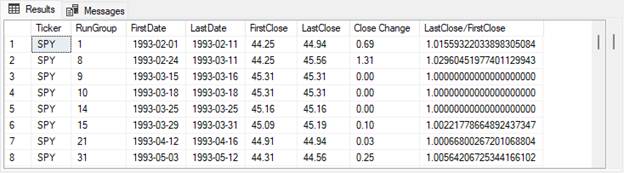
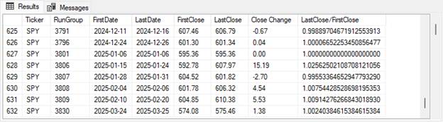
The following two screenshots display the first and last eight rows from the results set for the SPY ticker from the #temp_summary table. The results set for each ticker from the table appears in the order of the ticker values at the end of the preceding script.
· As you can see, there are a total of 632 RunGroups for the SPY ticker.
- The FirstDate and LastDate column values denote the beginning date and ending date for each RunGroup.
- The FirstClose and LastClose column values denote the beginning and ending close price for each RunGroup.
- The Close Change column values for each RunGroup equal the LastClose value less the FirstClose value.
- The LastClose/FirstClose column values for each RunGroup equals the LastClose value divided by the FirstClose value.
o When the column value equals 1, the LastClose value for a RunGroup precisely equals the FirstClose value.
o When the column value is less than 1, the FirstClose value is greater than the lastClose value.
o When the column value is greater than 1, the LastClose value is greater than the FirstClose value.
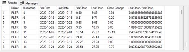
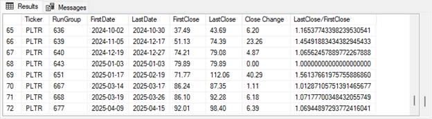
The next two screenshots show the first and last eight rows from the results set for the PLTR ticker. As you can see, there are a total of 72 RunGroups for the PLTR ticker. Column values are defined and can be interpreted according to the same rules as described for the SPY results set.
Comparison of Selected Backtest Results Across the Eight Tickers
This post aims to analyze and discuss the backtesting results of the Close_EMA_10_EMA_200 model for eight widely traded tickers. The model returns a set of distinct RunGroups for each ticker. The backtesting performance analysis focuses primarily on RunGroup and ticker combinations for which all trading days have a Close price that exceeds their corresponding EMA_10 and EMA_200 values.
A fundamental performance measure is the close price change from the first through the last trading day for each RunGroup within each ticker. The fundamental measure of performance is also impacted by the number of days over which a ticker is tracked. For these reasons, the fundamental measure is
- computed by both the median and mean across the RunGroups within each ticker and
- is also adjusted for the number of trading days over which each ticker is tracked.
This section also tracks the percentage of winning trades across each ticker where a trade is defined as a RunGroup. In general, a model that results in more trades with performance gains will be viewed more favorably than a model that results in less trades by a trader following recommendations from the model.
The tickers in this post divide naturally into two types.
- The first type is for tickers denoting leveraged and unleveraged ETFs. The SPY and SPXL tickers are both based on the S&P 500 index. The SPY ticker aims to return the daily percentage change as the S&P 500 index, and the SPXL ticker aims to return three times the daily percentage change as the S&P 500 index.
- Another pair of tickers belonging to the first ticker type are QQQ and TQQQ. These two tickers track the performance of the Nasdaq-100 index. The QQQ ticker aims to return the same daily percentage change as the Nasdaq-100 index, and the TQQQ ticker aims to return three times the daily percentage change as the Nasdaq-100 index.
- The second ticker type includes four very widely traded and leading security stocks. The tickers for these stocks are GOOGL, MSFT, NVDA, and PLTR. Two important ways that these tickers differ from first ticker types is that these tickers are for single stocks instead of a basket of securities, like an ETF. Additionally, these four tickers are all unleveraged.
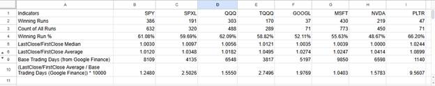
The following excerpt from a Google Sheets worksheet displays an overview of key performance indicators for each of the eight tickers analyzed via backtesting in this post. Rows 7 and 8 are hidden because their contents do not pertain to this post.
Rows 2 through 4 are counts and the percentage of winning model fits for each ticker’s model outcomes.
- A winning fit for a RunGroup is comprised exclusively of consecutive trading day outcomes with a TRUE CloseAboveEMA value. The counts in row 2 are the number of RunGroups for a ticker that are winning fits.
- The Count of All Runs in row 3 is the count of runs whether they have either TRUE or FALSE CloseAboveEMA values.
- The Winning Run % is the value in row 2 divided by the value in row 3 expressed in a percentage format. The ticker with the largest Winning Run % value is PLTR. This ticker is for a more recently introduced security than any of the other securities backtested in this post, but it returned a higher percentage of winning runs than any other ticker.
Rows 5 and 6 highlight the median and the average of the ratio between LastClose and FirstClose values across RunGroups for each ticker. Both the median and the mean serve as measures of central tendency, but the mean is more sensitive to extreme values. For the eight tickers analyzed as part of the backtest, the mean was consistently larger than the corresponding median for each ticker. This pattern indicates that the LastClose/FirstClose ratios are skewed toward larger values. Such skewness points to periods where closing prices increased significantly compared to opening prices, pulling the average upward while leaving the median less affected. This outcome highlights the impact of outliers for high-value Winning Run % values.
Finally, rows 6, 9, and 10 are for comparing growth across all tickers on a common scale. The base number of trading days is different for each of the tickers because the Google Finance site started tracking different tickers on different start dates. Furthermore, the base number of trading days can implicitly rescale the LastClose/FirstClose ratios across tickers.
- Row 9 contains the base number of trading days per ticker.
- Row 10 contains LastClose/FirstClose ratios from row 6 adjusted by the base number of trading days in row 9 and an arbitrary constant (10000) to control the number of places after the decimal point and facilitate comparisons in performance between tickers after adjusting for the base number of trading days per ticker.
- Here are a couple of take-aways from row 10.
o The two tickers for leveraged ETFs (SPXL and TQQQ) have substantially larger adjusted performance ratios than their matching unleveraged ETFs (SPY and QQQ).
o The PLTR ticker is associated with substantially superior adjusted performance ratios than other tickers for single stocks (GOOGL, MSFT, and NVDA) and ETFs (SPY, SPXL, QQQ, TQQQ). These performance ratio differences match the patterns for Winning Run % differences in row 4 -- PLTR has a higher value than any other ticker.
Concluding Comments
This post builds on a prior post that examines a buy-sell model for a pair of securities (SPY and SPXL). The main enhancement demonstrated in this post includes programmatically implementing the model so that it is easier and faster to compare more tickers and more trading days in backtesting analyses.
The analytics performed on the model outcomes in this post generated results that were generally consistent between percent winning trades and the ratio of FirstClose to LastClose values per RunGroup within each ticker. However, the model outcomes do not strictly represent ticker price performance. Instead, model outcomes reflect ticker price performance through the lens of the Close_EMA_10_EMA_200. Changing the model design can result in better or worse correspondence between the model and the historical price data. Therein lies the worth of being able to expedite model implementations via programming.
It is important to note that backtesting alone cannot guarantee future results for different stocks or time periods. However, well-constructed models that avoid overfitting can offer valuable insights—especially when historical data aligns with future conditions. Still, predictions remain subject to the inherent volatility of stock prices.
This post closes by noting that one of the innovations of this programmatic implementation of an analytical framework for a trading model can readily be adjusted for additional testing of different model assumptions.
- For example, different EMA period lengths can be compared to discover if other period lengths outperform the two examined in this post.
- The criteria for a winning trade can be readily modified. For example, we could change the definition of
o TRUE CloseAboveEMA column values so that rows are TRUE only when close prices are greater than these three matching EMAs (EMA_10, EMA_30, and EMA_50) and
o FALSE CloseAboveEMA column values so that rows are FALSE only when close prices are not greater than any of these three matching EMAs (EMA_10, EMA_30, and EMA_50).
- Additionally, the definition of TRUE and FALSE rows can be altered to depend on EMA crossovers for EMAs with different period lengths instead of the relationship of close prices to EMAs.


Comments
Post a Comment