Comparative Market Performance for a Buy-Sell Model Versus a Buy-and-Hold Strategy for Eight Tickers
The last couple of Security Trading Analytics blog posts introduced and examined the logic of a buy-sell model based on close prices and two exponential moving averages (EMAs). The first post pulled data from the Google Finance site and showed how to implement the model manually within a Google Sheets workbook for two tickers (SPY and SPXL) over a couple of different timeframes. The second post illustrated how to use T-SQL to programmatically implement the buy-sell model and perform backtests from their original close price with a Google Sheets workbook of the model for eight tickers (SPY, SPXL, QQQ, TQQQ, GOOGL, MSFT, NVDA, and PLTR). The current post compares the market performance of the buy-sell model to a buy-and-hold strategy for the eight tickers in the second post. All eight tickers in this post are compared from the first trading date in 2021 through April 15, 2025, the closing date in the second prior post.
There are four key sections and some concluding comments to this post. The first section reviews the buy-sell model mechanics. The second section describes how to compute market performance for a buy-and-hold strategy. The third section describes how to compute market performance for the buy-sell model. The fourth section compares the market performance outcomes for each ticker from the buy-and-hold strategy versus the buy-sell model. Finally, the concluding comments at the end of this post discusses how self-directed traders and stock market analysts can easily augment their existing trading strategies with the buy-sell model. The concluding comments also describe possible next steps in the evolution of the buy-sell model and calls for any input you care to offer.
A Review of the Buy-Sell Model Mechanics
This post assigns a name of Close _EMA_10_EMA_200 to the buy-sell model. An EMA is a smoothing technique for an underlying time series, such as close prices for a ticker. The trailing number for an EMA denotes the period length for an EMA. An EMA with a small trailing number, such as EMA_10, reflects recent underlying price trends. In contrast, an EMA with a relatively large trailing number, such as EMA_200, reflects less recent underlying price trends. The first prior post for this post demonstrates how to compute EMA_10, EMA_30, EMA_50, and EMA_200 time series values that are for an underlying close price series.
When the close price is greater than EMA_10 and EMA_200 for a series of consecutive trading days, then the close prices are trending up over both the short-term and the long-term. By contrast, when the close price is not greater than EMA_10 and EMA_200 for a series of consecutive trading days, then the close prices are not trending up.
A period of consecutive trading days when close prices are trading up is called a RunGroup. There are also RunGroups for consecutive trading days when close prices are not trending up. Each RunGroup has a unique numerical identifier whether it is for a set of consecutive trading days that are trending up or not trending up.
The Close _EMA_10_EMA_200 model assumes that consecutive periods with upward trending close prices will lead to more periods with upward trending close prices until they do not. For example, a string of consecutive trading days with upward trending close prices will have a higher close for the last trading day in the consecutive series than the first trading day in a series. Therefore, the buy-sell model prescribes that you buy at the first trading day where the close price exceeds both EMA_10 and EMA_200. The model also prescribes that the security for a ticker should be sold on the day before the close price series flips from trending up to not trending up.
Computing Ticker Market Performance for a Buy-and-Hold Trading Strategy
This section shows three excerpts from a Google Sheets workbook that was used to support the second prior post for the current post. The excerpts are to clarify the process for computing market performance from the first trading day in 2021 (January 4, 2021) through April 15, 2025 for the close prices for a ticker (SPY). By computing the market performance for a standard date range, this post can compare market performance both across tickers as well as across different trading strategies, such as buy-and-hold versus buy-and-sell based on the relationship of close prices to EMA values.
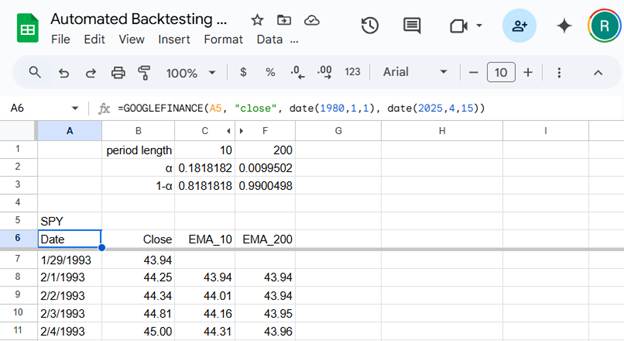
The following screenshot shows the first several rows of time series data for the SPY ticker. Column A starting in row 7 stores date values from the Google Finance site. SPY close values are extracted from the Google Finance site to a Google Sheets worksheet. The expression for the transfer of the close values is in cell A6. The GOOGLEFINANCE function in cell A6 has four parameters.
A5 points to cell A5, which contains a string value for the SPY ticker.
The string value “close” tells the Google Finance site to return just close values as opposed to open, high, or low values, for the ticker in the function’s first parameter value.
The date function expression date(1980,1,1) tells Google Finance to return close values starting as soon as January 1, 1980 or the first available date after that date. The screenshot below shows the first available date from Google Finance for the SPY ticker is January 29, 1993. The start date for close price time series varies depending on when the Google Finance started tracking close prices for a ticker.
The date function date(2025,4,15) specifies the most recent date (April 15, 2025) through which the second prior post to the current post collects time series data from Google Finance. Time series data are collected for all eight tickers for this same date.
Because the starting dates for close price time series values can vary substantially from one ticker to another, it is useful to analyze extracted data on a common timeframe for which all tickers can be compared. It turns out that all eight tickers examined in this post (and the second prior post to this post) have close time series values from the first trading date in 2021(January 4, 2021) through April 15, 2025. Therefore, the post compares tickers over this date span.
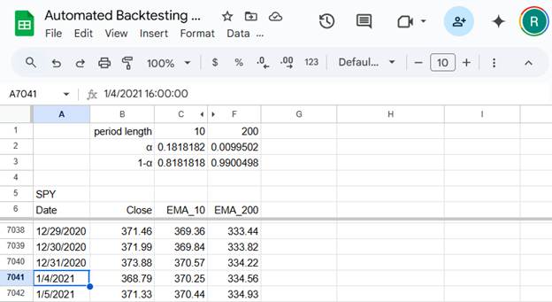
The following screenshot shows the first trading date in 2021 selected for a worksheet with SPY data. Notice the trading date appears right after December 31, 2020 is January 4, 2021. This confirms that January 4 is the first trading date in 2021.
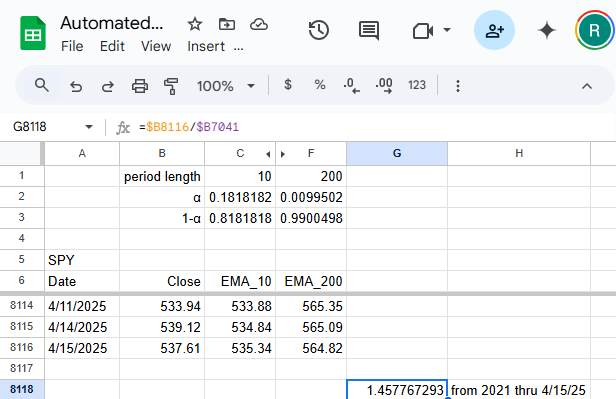
The third screenshot in this section shows three rows of data through the last date tracked (April 15, 2025) in this post for close values in 2025. The expression in cell G8118 computes the ratio of the most recently tracked close price on April 15, 2025, divided by the first tracked close price on January 4, 2021. The ratio in cell G8118 reflects the growth in close prices from the first through the most recently tracked date. The ratio is computed as the close value in cell B8116 divided by the close value in cell B7041, which is the close price on January 4, 2021. The ratio value of 1.457767293 indicates close prices grew by slightly more than 45 percent for the SPY ticker from the first through the last tracked date with the buy-and-hold strategy.
This post repeats the process for buy-and-hold growth rates for the SPY ticker for the remaining seven tickers tracked in this post.
Computing Ticker Market Performance for the Close _EMA_10_EMA_200 Model
As indicated in the “A Review of the Buy-Sell Model Mechanics” section, the Close _EMA_10_EMA_200 model recommends buying at the first date in an upward trending RunGroup and selling at the last date in an upward trending RunGroup. Furthermore, the model does not recommend trading a ticker’s security during a RunGroup that is not upward trending.
As a consequence of these guidelines, the first step in computing market performance for the Close _EMA_10_EMA_200 model is to filter for only upward trending RunGroups. The T-SQL script that implements the buy-sell model returns a seven-column results set for each ticker’s data that is submitted to it. The results set for each ticker is, in turn, used to populate a worksheet in a Google Sheets workbook. Analyses can then be performed from within the worksheet for each ticker.
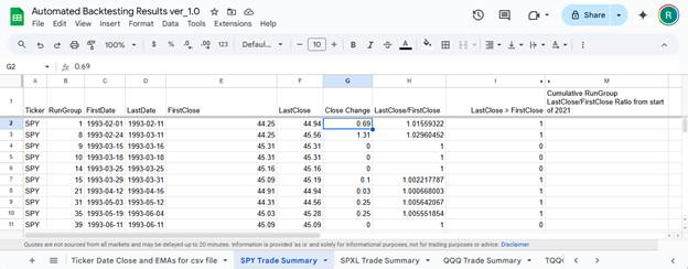
The following screenshot shows the first ten rows for the SPY Trade Summary worksheet in the Automated BackTesting Results ver_1.0 workbook. Columns A through G are copied from the results set output for the SPY ticker.
Column A denotes the ticker for which data is output.
Column B displays the RunGroup numerical identifier for a row.
Columns C and D are, respectively, for the first and last dates of the RunGroup displayed in a row.
Columns E and F are, respectively, for the first and last close prices of the RunGroup displayed in a row.
Column G is the close price change of the RunGroup displayed in a row.
The remaining three displayed columns (H, I, and M) are computed through expressions within the worksheet. The rows for the last column (M) are not populated in the following worksheet image because they do not pertain to RunGroups whose first and last are from within January 4, 2021, through April 15, 2021; recall that these dates are for the market performance date range in the current post.
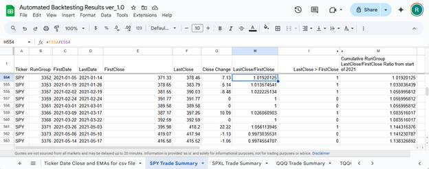
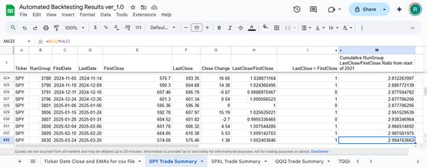
The next pair of worksheet excerpts are for SPY cumulative market performance computations. The first member of the pair shows the data for the first ten rows in the market performance evaluation timeframe (from January 4, 2021, through April 15, 2025). The second member of the pair shows the data for the last ten rows in the market performance evaluation timeframe.
In the first pair member, the cursor rests in cell H554. This cell contains an expression that computes the last close value divided by the first close value for the first RunGroup in the performance evaluation timeframe; the numerical identifier for this RunGroup is 3352. Notice that the FirstDate value for the first row has a value of 2021-01-05, which is one day after the start of performance evaluation timeframe. The LastDate value (2021-01-14) for the first row is the ninth calendar day after the start of the first RunGroup in the evaluation timeframe.
Cell H554 shows the ratio of the LastClose value divided by the FirstClose value for the first Run Group. Notice also that column M for row 554 has the exact same value as column H for row 554. This relationship is not maintained in the second row of the first pair member below. That is because column H shows its ratio for the current row in the worksheet, but column M shows its ratio for the cumulative value for a RunGroup. The cumulative LastClose/FirstClose ratio for the second RunGroup equals 1.01920125 multiplied by 1.013574541, which equals 1.033036439.
The cumulative LastClose/FirstClose ratio value (2.994763663) in the last row in column M of the second pair member is especially significant. This is the compound ratio value from the first RunGroup in row 554 through the RunGroup in the last row within the evaluation timeframe – namely, row 633. In other words, the ratio value in M633 is the compound ratio value from the FirstClose in row 554 through the LastClose value in row 633 for the SPY Trade Summary worksheet.
This post repeats the process for buy-sell growth rates for the SPY ticker for the remaining seven tickers tracked in this post.
Market Performance for Buy-and-Hold Strategy Versus the Buy-Sell Model
The following table presents market performance results on a total change basis and an average annual change basis for the buy-and-hold strategy versus the buy-sell model. The change percentages are displayed individually for each of the eight tickers examined in this post.
Here are some highlights from the following table.
The improvement for the buy-sell model relative to the buy-and-hold strategy on an annual basis is substantial, ranging from a low of 35.88% for SPY to a high of 1663% for PLTR.
The average annual percentage improvement per year for both NVDA and PLTR tower above the improvement for other securities (SPY, SPXL, QQQ, TQQQ, GOOGL, and MSFT).
It is also true that leveraged ETFs, such as SPXL and TQQQ, exhibit superior market performance relative to ETFs based on analogous indexes that are not leveraged, such as SPY and QQQ.
The buy-sell model has a couple of distinct tactical advantages that support its superior performance relative to a buy-and-hold strategy.
The buy-sell model can exit a ticker position when the likelihood of near-term future gains reduce, and then re-enter a ticker position later when the likelihood of near-term future gains increase. The greater the number and durations of holding periods, the better the performance of a buy-sell model. Typical holding periods may be days, weeks, or even months.
The buy-and-hold strategy holds a ticker position from its open date through to its close date no matter whether a ticker price is rising or falling in the near term. The strategy assumes the likely error in estimating near-term future gains is so large that it cannot be profitable to enter and exit trades based on estimated near-term gains. Therefore, the buy-and-hold strategy selects tickers based on long-term criteria, which do not necessarily change in the near term. Typical holding periods may be many months, years, or even decades.
Additionally, the buy-sell model can compound changes between consecutive holding periods. When the buy-sell model generates multiple successful trades, then it’s total change is the compounded change across those trades. This compounding effect further contributes to the tactical advantage of a buy-sell model relative to a buy-and-hold strategy.
Concluding Comments
This post builds on a pair of prior posts (“Building and Backtesting a Buy-Sell Model with Close Prices and EMAs” and “Programming and Backtesting Demonstrations for a Buy-Sell Model for Eight Tickers”) for a buy-sell model. The main enhancement demonstrated in this post is the comparison of the buy-sell model to a buy-and-hold strategy over a common timeframe. The post also describes a comparison technique for any buy-sell model to a buy-and-hold strategy. The buy-sell model examined in this post for eight tickers substantially outperformed a buy-and-hold strategy.
Self-directed traders and stock market analysts can perform ad hoc manual assessments of the model with any charting package that can display close prices for tickers along with ten-day and two-hundred-day exponential moving averages. Finviz and StockCharts.com are two widely used packages that support this kind of functionality. I use Finviz to evaluate setups for my daily trading decisions with live trading data, and I regularly view videos on by leading stock market strategists where charts from StockCharts.com are frequently used.
This post concludes with a request for preferences for next steps for the buy-sell model described in this post. Vote by leaving a comment for suggested next steps below.
Would you like to see an application and evaluation of the buy-sell model for different asset types, such as tickers for precious metals, cryptocurrencies, or semiconductor and AI firms? If you vote for this option, please list specific tickers that you want analyzed.
Would you like to see how different EMAs perform in the buy-sell model, such as EMA_5, EMA_8, EMA_20, EMA_30, EMA_50, EMA_100, and EMA_150?
Would you like to see future posts examine different criteria, such as the (Close > EMA_10, Close > EMA_200, and EMA_10 > EMA_200) or excluding Close from the criteria set for buy-sell decisions?
Any other preferred next step that interests you the most?
Keywords: ##BuySellModel, ##BuyAndHoldStrategy, ##ClosePrices, ##ExponentialMovingAverages, ##TotalChange, ##AverageAnnualChange,##BuySellPercentImprovement, ##SPY, ##SPXL, ##QQQ, ##TQQQ, ##GOOGL,##MSFT, ##NVDA, ##PLTR


Comments
Post a Comment